DataEng: GCP: Loading data with Google Datalab Python BigQuery (bq) Part 2

Continue from Part 1


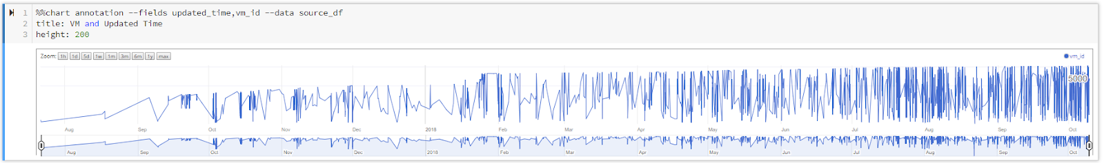
Taking previous work from Part 1, this will continue to cleansing and transforming the data which include numpy libraries.

Setting up indicators with Panda

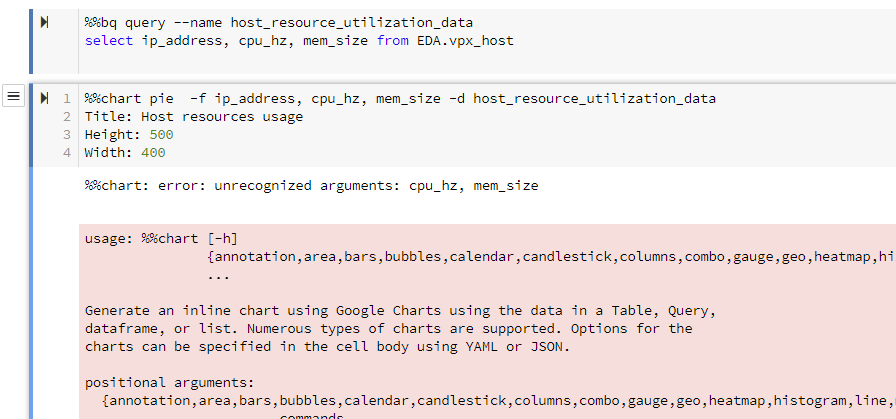
import google.datalab.bigquery as bq
import numpy as np
import pandas as pd

bq_vm = bq.Query('SELECT * FROM EDA.vpx_vm')
output_opt = bq.QueryOutput.table(use_cache=False)

##Print result set
raw = bq_vm.execute(output_options=output_opt).result()
source_df = raw.to_dataframe()

# getting vm_id column as indicator variable with panda
source_df = pd.concat([source_df, pd.get_dummies(source_df['vm_id'],prefix='Column_vm_id')],axis=1)
source_df = pd.concat([source_df, pd.get_dummies(source_df['updated_time'],prefix='Column_updated_time')],axis=1)
source_df.head(9)

Describe() and Corr()

import google.datalab.bigquery as bq
import numpy as np
import pandas as pd
#Prerequisite - Load or create the table to BigQuery Dataset first.
bq_vm = bq.Query('SELECT * FROM EDA.vpx_vm')
output_opt = bq.QueryOutput.table(use_cache=False)

##Print result set
raw = bq_vm.execute(output_options=output_opt).result()
source_df = raw.to_dataframe()

# getting vm_id column as indicator variable
source_df = pd.concat([source_df, pd.get_dummies(source_df['vm_id'],prefix='Column_vm_id')],axis=1)
source_df = pd.concat([source_df, pd.get_dummies(source_df['updated_time'],prefix='Column_updated_time')],axis=1)

#source_df.head(9)

#The describe will take longer.
#It comes up with count, mean, standard deviation, minimum, percentiles and max.
#source_df.describe()

#this will take a long time.
source_df.corr()['ds_id']

Saving the results in the bucket - Cloud Storage

import google.datalab.bigquery as bq
import numpy as np
import pandas as pd
from StringIO import StringIO

#Prerequisite - Load or create the table to BigQuery Dataset first.

bq_vm = bq.Query('SELECT * FROM EDA.vpx_vm')

output_opt = bq.QueryOutput.table(use_cache=False)

##Print result set
raw = bq_vm.execute(output_options=output_opt).result()
source_df = raw.to_dataframe()

# getting vm_id column as indicator variable
source_df = pd.concat([source_df, pd.get_dummies(source_df['vm_id'],prefix='Column_vm_id')],axis=1)
source_df = pd.concat([source_df, pd.get_dummies(source_df['updated_time'],prefix='Column_updated_time')],axis=1)

#source_df.head(9)

#The describe will take longer.
#It comes up with count, mean, standard deviation, minimum, percentiles and max.
#source_df.describe()

#this will take a long time.
#source_df.corr()['ds_id']

#saving the results to Cloud Storage
csvObj=StringIO()
source_df.corr()['ds_id'].to_csv(csvObj)

Creating csv file in GCS Bucket

%%gcs write --variable csvObj --object 'gs://datalab-project-1-239921/storing_correlation_data.csv'

The gcs write will create the new csv file in the GCS Bucket.

I am lacking meaningful data to play with especially in the Correlation and Std Deviation parts. Though, the GCS APIs worked.

DataEng: GCP: Datalab cheatsheet

datalab create datalab-project-1

datalab connect datalab-project-1

--stop and stop the billing
datalab stop datalab-project-1

-- list datalab projects
datalab list

--delete the datalab instance
datalab delete -delete-disk 

pic

DataEng: GCP: Loading data with Google Datalab Python BigQuery (bq) Part 1

https://googledatalab.github.io/pydatalab/datalab.bigquery.html


Prerequisite
The vpx_vm table must be uploaded to BigQuery Dataset already. Otherwise, the code will throw an exception "Exception: notFound: Not found: Table .. . .. not found in location ..

"

Performing a Select Count(*) on vpx_vm table.

#Template

import google.datalab.bigquery as bq
# query
bq_vm = bq.Query('SELECT count(*) FROM EDA.vpx_vm')
output_opt = bq.QueryOutput.table(use_cache=False)

#executing the query statement
result = bq_vm.execute().result()

##Print result set
raw = bq_vm.execute(output_options=output_opt).result()
source_df = raw.to_dataframe()
print (source_df)

#Print result set all in a line.
resultset = bq_vm.execute(output_options=output_opt).result().to_dataframe()
print (resultset)

    f0_
0  4258
    f0_
0  4258

Build upon from the template.

import google.datalab.bigquery as bq

bq_vm = bq.Query('SELECT * FROM EDA.vpx_vm')

output_opt = bq.QueryOutput.table(use_cache=False)
raw = bq_vm.execute(output_options=output_opt).result()

source_df = raw.to_dataframe()
print('Column             Data type ')
source_df.dtypes

Column               Data type 







vm_id                int64
ds_id                  int64
updated_time    datetime64[ns]
dtype: object

Perform select all on the table.

import google.datalab.bigquery as bq

bq_vm = bq.Query('SELECT * FROM EDA.vpx_vm')
## simply printing the statement out.
print (bq_vm)
print ('\n')

output_opt = bq.QueryOutput.table(use_cache=False)
#print (output_opt)


#result = bq_vm.execute().result()
#print (result)

##Print result set
raw = bq_vm.execute(output_options=output_opt).result()
source_df = raw.to_dataframe()
print (source_df)

BigQuery Query - SELECT * FROM EDA.vpx_vm

      vm_id  ds_id            updated_time
0        27   4098 2018-08-21 22:05:03.437
1       213   4098 2018-08-21 22:05:04.547
2       730   4098 2018-08-21 22:05:05.440
3       799   4098 2018-08-21 22:05:02.933
4       907   4098 2018-08-21 22:05:05.123
5      1006   4098 2018-08-21 22:05:06.153
6      1018   4098 2018-08-21 22:05:05.367
7      1019   4098 2018-08-21 22:05:04.040
8      1022   4098 2018-08-21 22:05:03.937
9      1041   4098 2018-08-22 18:02:38.317
10     1059   4098 2018-08-21 22:05:06.230
11     1162   4098 2018-08-21 22:05:06.063

Using

source_df.head() to get the following results.

In comparison, BigQuery is a lot more natural than Panda where the Python Panda API is heavily used. Database operation can easily fit into the BigQuery.Query API. Both are easily integrate with GCP Chart. Basically, the charting can be done with BigQuery, Python BigQuery API or Panda.


BigQuery

%%bq query --name host_resource_by_ip_sum_data

select ip_address, sum(cpu_hz) as SUM_CPU, sum(mem_size) as  SUM_MEMORY from EDA.vpx_host group  by ip_address

Python BigQuery

#Template
import google.datalab.bigquery as bq
# query
bq_vm = bq.Query('SELECT count(*) FROM EDA.vpx_vm')
output_opt = bq.QueryOutput.table(use_cache=False)

Python Panda

import pandas as pd
from StringIO import StringIO
#create dataframe
vm_df = pd.read_csv(StringIO(vpx_vm_data))
date_summary=vm_df.groupby(['updated_time'],as_index=False)['vm_id'].sum()
print(date_summary.head())
date_summary['updated_time'] = pd.to_datetime(date_summary['updated_time'])
date_summary.dtypes

DataEng: GCS: Experimenting Panda operations.

Playing with Panda APIs


How the full dataset looks like

import pandas as pd
from StringIO import StringIO
#create dataframe
data = pd.read_csv(StringIO(vpx_vm_data))
print(data)

      vm_id  ds_id                   updated_time
0        27   4098  2018-08-21 22:05:03.437000000
1       183    166  2018-10-08 14:43:10.690000000
2       184    172  2017-10-03 15:59:10.957000000
3       185    162  2017-10-04 01:46:15.417000000
4       187   4924  2017-11-28 21:11:14.127000000
5       188    165  2018-04-23 14:22:01.403000000
6       190    158  2017-10-03 18:00:11.513000000
7       192    173  2018-10-08 21:28:54.837000000
8       193   4100  2018-07-31 21:17:10.343000000
9       194   4925  2017-11-30 17:35:31.977000000
10      196    164  2018-07-08 01:41:37.240000000
11      198    162  2017-10-04 01:46:15.450000000
12      199   4924  2018-04-19 18:15:00.330000000
13      201    169  2018-04-23 14:21:37.287000000
14      203    157  2017-11-07 02:05:28.810000000
15      205    168  2018-02-09 19:31:50.713000000
16      207    158  2017-10-03 15:59:10.363000000
17      208    170  2017-10-03 20:32:52.197000000
18      209    168  2017-10-03 18:00:10.777000000
19      210    169  2017-12-19 14:30:03.007000000
20      211   4100  2018-08-31 16:10:02.320000000
21      212   4098  2018-08-21 22:05:04.547000000
22      213   4065  2018-07-30 21:07:11.120000000
23      214    167  2017-10-03 18:20:18.003000000
24      216   4924  2018-09-25 21:33:04.523000000
25      217    158  2018-04-23 14:20:04.123000000
26      218   5046  2018-04-19 18:14:37.350000000
27      221   4925  2018-08-02 18:37:33.573000000
28      239   6868  2018-05-25 02:55:54.327000000
29      242    158  2018-10-05 21:00:12.307000000
...     ...    ...                            ...
4228   7571   4061  2018-09-24 15:32:39.943000000

counts(*)

import pandas as pd
from StringIO import StringIO
#create dataframe
vm_df = pd.read_csv(StringIO(vpx_vm_data))
date_summary=vm_df.count()
print(date_summary.head())

vm_id           4258
ds_id           4258
updated_time    4258
dtype: int64

That is equivalent to the following. It represents all the columns in the same counts.

select count(*) from vpx_vm;

count(vm_id)

import pandas as pd
from StringIO import StringIO
#create dataframe
vm_df = pd.read_csv(StringIO(vpx_vm_data))
date_summary=vm_df[['vm_id']].count()
print(date_summary.head())

vm_id    4258
dtype: int64

That is equivalent to the following

select count(vm_id) from vpx_vm;

Count with every single column.

import pandas as pd
from StringIO import StringIO
#create dataframe
vm_df = pd.read_csv(StringIO(vpx_vm_data))
date_summary=vm_df.groupby('vm_id').count()
print(date_summary)

That is equivalent to the following.

select vm_id, count(vm_id), count(ds_id), count(updated_time) from EDA.vpx_vm group by vm_id, ds_id, updated_time order by vm_id;

Sorting and Where clause

import pandas as pd
from StringIO import StringIO
#create dataframe
data = pd.read_csv(StringIO(vpx_vm_data))
##print (data)
print data.sort_values("vm_id", inplace=True)
data.where(data["vm_id"]==183, inplace = True)
##data.where(data["vm_id"]==183, inplace = True) --this will spit out everything.
print (data)

None
      vm_id  ds_id                   updated_time
0       NaN    NaN                            NaN
1     183.0  166.0  2018-10-08 14:43:10.690000000
2       NaN    NaN                            NaN
3       NaN    NaN                            NaN
4       NaN    NaN                            NaN
5       NaN    NaN                            NaN
6       NaN    NaN                            NaN
7       NaN    NaN                            NaN
8       NaN    NaN                            NaN
9       NaN    NaN                            NaN
10      NaN    NaN                            NaN
11      NaN    NaN                            NaN
12      NaN    NaN                            NaN
13      NaN    NaN                            NaN
14      NaN    NaN                            NaN

Note 1: data.where(data["vm_id"]==183, inplace = True) is comparison to an integer. data.where(data["vm_id"]=="183", inplace = True) , is comparing to a string and it will fail with error "TypeError: invalid type comparison".

Note 2: inplace = True is used to 'masked' out. Those "NaN" are the result of inplace sets to Tru

That's is similar to the following.

select vm_id, ds_id, updated_time from EDA.vpx_vm where vm_id=183 order by vm_id;

DataEng: GCS: Data Visualizing with %%chart

What good will it do if one can't visualize and picture the data? Visualizing the data can be achieved from BigQuery -Data Studio or Datalab - %%chart function. In this blog, I am going to try out visualizing the data with Datalab - %chart feature.


[Learned]
variables CANNOT have space in between. Otherwise, it would error out with "%%chart: error: unrecognized arguments: "


[Learned] 
The Title, Height, Width should be "title", "height" and "width" respectively. It is case sensitive. Why didn't GCS provide better hints or indications on these?  Submitted recommendation to GCP on this.

Charting with Pie

%%bq query --name host_resource_utilization_data
select ip_address, cpu_hz, mem_size from EDA.vpx_host

%%chart pie  -f ip_address,cpu_hz,mem_size -d host_resource_utilization_data
title: Host resources usage
height: 1000
width: 1000

Pie Chart with each IP with total resources used. Using SUM to group by.

%%bq query --name host_resource_by_ip_sum_data
select ip_address, sum(cpu_hz) as SUM_CPU, sum(mem_size) as SUM_MEMORY from EDA.vpx_host group  by ip_address

%%chart pie  -f ip_address,SUM_CPU,SUM_MEMORY -d host_resource_by_ip_sum_data
title: Host resources usage by IP address
height: 1000
width: 1000

Charting with line where the axis X represents IP address and the lines are CPU and Memory.

%%chart line -f ip_address,cpu_hz,mem_size -d host_resource_utilization_data
height: 300

Charting in Histogram but not very meaningful here.

%%bq query --name host_resource_by_ip_histogram_data
select ip_address,cpu_hz from EDA.vpx_host

%%chart histogram -f ip_address,cpu_hz -d host_resource_by_ip_histogram_data
title: Host Resources Usage in Pie Chart
height: 1000
width: 1000

Charting with Timelined.


Load vpx_vm.csv with extracted data with the following query to GCS Bucket

select vm_id, ds_id, updated_time from vpx_vm_ds_space;

%%gcs read --object 'gs://datalab-project-1-239921/vpx_vm.csv' --variable vpx_vm_data

Example of using panda and Dataframe.

import pandas as pd
from StringIO import StringIO
#create dataframe
vm_df = pd.read_csv(StringIO(vpx_vm_data))
date_summary=vm_df.groupby(['updated_time'],as_index=False)['vm_id'].sum()
print(date_summary.head())
date_summary['updated_time'] = pd.to_datetime(date_summary['updated_time'])
date_summary.dtypes

That is equivalent to the following query. Apparently, not very meaningful.

select sum(vm_id), updated_time from EDA.vpx_vm group by updated_time;

%%chart annotation --fields updated_time,vm_id --data date_summary
title: VM and Updated Time
height: 200

DataEng: GCS: Connect to Datalab

Before working on Jupyter Notebook where it hosts by Datalab Computer Engine, the user must connect to it first.


To list projects under an account.
Command: Datalab list

C:\Users\xxxxxxxx\AppData\Local\Google\Cloud SDK>datalab list
NAME                ZONE           MACHINE_TYPE   PREEMPTIBLE  INTERNAL_IP  EXTERNAL_IP  STATUS
datalab-kl-project  us-central1-c  n1-standard-1               10.128.11.12                TERMINATED

Terminate indicating the project stopped. This is different than project doesn't exist. (another blog shows more detail on how to start the project.)

Command: datalab connect <datalab_name> --port <port_num>
Example: datalab connect datalab-kl-project --port 8123

Note: Datalab name is not Project Name. 

[Learned]

Error: (gcloud.compute.onstances.list) Some requests did not succeed:
 - Failed to find project datalab-1-123456

A nested call to gcloud failed, use --verbosity=debug for more info.

This means the project is NOT currently existed or it has been shutdown and staying in Pending To Delete section. It needs to be created or restored from the pending to delete list It needs to be started from the GCP Console. Once the project is started, the Billing needs to be enabled for the project. Perform a search on the project again. At this point, GCP seems to have little glitches in the Compute Engine saying, unable to locate the resource or project even though it has been started.


[Learned]
There might be a possibility that Firewall will prevent the ability to connect to the GCP. If disabling the firewall is possible, perform it temporarily for the connectivity to happen. If it connects successfully, it will look similar to the following.

There might not be a specific error message related to security but will look like the following messages.

Waiting for Datalab to be reachable at http://localhost:8123
Timeout waiting for the connection to become healthy.Trying again with a new connection...
Connection closed
Attempting to reconnect...
Waiting for Datalab to be reachable at http://localhost:8123
.....

If it connects without incidents, it should look like the following and the Datalab and Jupyter Notebook is ready.

C:\> datalab connect datalab-kl-project --port 8123
Connecting to datalab-kl-project.
This will create an SSH tunnel and may prompt you to create an rsa key pair. To manage these keys, see https://cloud.google.com/compute/docs/instances/adding-removing-ssh-keys
Waiting for Datalab to be reachable at http://localhost:8123/

The connection to Datalab is now open and will remain until this command is killed.
You can connect to Datalab at http://localhost:8123/

DataEng: GCS: List, Shutdown and Restore gcs project from gcloud

Another option I used to list, shutdown and restore Project to prevent credits from going over the limit quickly.

C:\Google\Cloud SDK>gcloud projects list
PROJECT_ID                NAME               PROJECT_NUMBER
datalab-project-1-239921  DataLab Project 1  2334346706279
C:\Google\Cloud SDK>gcloud projects delete datalab-project-1 datalab-project-1-239921

Once deleted the VM, Compute Engine and etc associated with the project will no longer be accessible. The Billing will also indicate the project no longer linked to it. The project will stay roughly 30 days before it is purged away.


The Jupyter Notebook will almost immediately throw an error.

The Billing will unlink the project.

Billing Overview should show no linked project instead of a project linked to it with charges.

Note: as of to date., there is no way to query the projects that are sitting in the "Resources pending deletion" section with gcloud command line. User will need to view that from the gcloud Console.


In order to restore, use the following command line.

C:\Google\Cloud SDK>gcloud projects undelete datalab-project-1 datalab-project-1-239921

C:\Google\Cloud SDK>gcloud projects undelete datalab-project-1-239921
Restored project [https://cloudresourcemanager.googleapis.com/v1/projects/datalab-project-1-239921].

User may still need to get back into the Console to enable/change the billing to the project then start the datalab again. These 3 steps work the same as first creating a project for Datalab.

DataEng: GCS: retrieving information from Bucket objects with gcs command and python API

Retrieving information from the bucket can be achieved with either through gcs command line or google lab python API.

import google.datalab.storage as storage

#Create an object for the specific bucket
bucket_object = storage.Bucket('datalab-project-1-239921')

#iterate through the objects and print them
for obj in bucket_object.objects():
    print(obj.key)

DataEng: GCS: Loading Table to BigQuery

In this blog, I exported partial records from a vCenter schema from SQL Server with the following query on VPX_HOST and created a vpx_host.csv document.

select  ip_address, cpu_hz, mem_size from EDA.vpx_host

From the GCP Console, go down to BigQuery and click into it.

First, create a Dataset then create a table within it. Once the table is created, it can be queried just like normal RDBMS.


[Learn] 
The query output is cached. Say, if I have version 1 VPX_HOST table created, then I modified the CSV, deleted the BiqQuery table and upload a new one. running a query will still presenting old dataset. In order to start from a fresh query, user need to click on the upper right-hand button - "+ COMPOSE NEW QUERY"

That's it, on how to create Table in BiqQuery. I will utilize this data loading for my data visualization blog. Before visualizing the data with charts, I need to load the table with data first.
[Go to Data Vizualization]

DataEng:GCS: Datalab Timeout

Datalab can timeout if unattended for a bit of time.

Notebook for the GCP Datalab session will timeout as well.

Reconnect to the GCP Datalab. There is not Reconnect feature but Connect.

datalab connect datalab-kl-project --port 8123

All the timeout sessions in the Jupyter Notebook will need to be reinitiated. They cannot be reused.

DataEng: GCS: Writting contents into GCP Bucket

Prior to writing an object to the Bucket, it is a good idea to verify what's in it first.

This can be achieved by using gsutil utility from activating Cloud Shell.

xxxxx@cloudshell:~ (datalab-project-1-239921)$ gsutil ls -l
gs://datalab-project-1-239921/
gs://test-create-bucket-2-32321/
xxxxx@cloudshell:~ (datalab-project-1-239921)$ gsutil ls -l gs://test-create-bucket-2-32321/
  76398379  2019-05-10T21:23:46Z  gs://test-create-bucket-2-32321/Events_Export.csv
      7340  2019-05-10T21:47:55Z  gs://test-create-bucket-2-32321/entity.csv
TOTAL: 2 objects, 76405719 bytes (72.87 MiB)
xxxxx@cloudshell:~ (datalab-project-1-239921)$

Executing the data insertion in Jupyter Notebook, this will create an insert-text.text with text in it.

xxxxx@cloudshell:~ (datalab-project-1-239921)$ gsutil ls -l gs://test-create-bucket-2-32321/
  76398379  2019-05-10T21:23:46Z  gs://test-create-bucket-2-32321/Events_Export.csv
      7340  2019-05-10T21:47:55Z  gs://test-create-bucket-2-32321/entity.csv
        13  2019-05-13T21:06:30Z  gs://test-create-bucket-2-32321/insert-text.text
TOTAL: 3 objects, 76405732 bytes (72.87 MiB)

xxxxx@cloudshell:~ (datalab-project-1-239921)$gsutil cat gs://test-create-bucket-2-32321/insert-text.text
Inserted text

DataEng: GCS: DataStudio

What is Data Studio? Basically, data visualization tool similar to Datalab Chart.

DataEng: GCS: BigQuery

BigQuery can be performed in the Console's BigQuery or through Jupyter Notebook. Prior to performing a query from Jupyter Notebook, a user might want to make sure if the table even existed first as Jupyter Notebook will not provide any indication if the table doesn't exist [Learn].

The following example indicating that in my Dataset, I do not have any tables. Even though I can perform a query on Jupyter Notebook, it would not error out.

DataEng: GCS: Shutting down project

For those who are using Trial account might need to be more cautious of not having the project runs continuously where it will slowly eating up the credits.

From the Search bar, type Project and click on the project on the Compute Engine.

Upon shutting down the Project, accessing it through the Jupyter Notebook may trigger dialogue windows such as below. Connecting from GCS SDK Console would fail as well.

User can go back to the Billing from the Console to verify nothing is charged or active. This will essentially put the project and all the resources (Computer Engine and etc) into delete mode and will be removed from the account in 30 days if the user is not restoring and starting it. On how to restore and starting, the user can check out this blog. https://dataengineeringdesk.blogspot.com/2019/05/dataeng-gcs-starting-project.html

DataEng: GCS: Starting Project

Upon listing availability of any projects, I am getting the following output. The Status is Terminated. What this means is, the project exists but shutdown.

Internal_IP has been masked out. It should present an Internal IP address.

Start the project from GCP Console

I am prompted with billing which I have enabled earlier when restoring the Project.

The grayed icon should turn to green and the project is started.

Datalab list will show Internal IP, External IP and the status is "RUNNING"